Reintroducing tsibble: data tools that melt the clock
Preface
![]()
I have introduced tsibble before in comparison with another package. Now I’d like to reintroduce tsibble (bold for package) to you and highlight the role tsibble (italic for data structure) plays in tidy time series analysis.
The development of the tsibble package has been taking place since July 2017, and v0.6.2 has landed on CRAN in mid-December. Yup, there have been 14 CRAN releases since the initial release, and it has evolved substantially. I’m confident in the tsibble’s data structure and software design, so the lifecycle badge has been removed, thus declaring the maturity of this version.
Motivation

Figure 1: Can we flatten the lumpy path of converting raw temporal data to model-ready objects?
If data comes with a time variable, it is referred to as “temporal data”. Data arrives in many formats, so does time. However most existing time series objects, particularly R’s native time series object (ts), are model-focused assuming a matrix with implicit time indices. Figure 1 expresses the lumpy path to get from wild temporal data into model-ready objects, with myriads of ad hoc and duplicated efforts.
However, the temporal data pre-processing can be largely formalised, and the tools provided by tsibble do this, and more. It provides tidy temporal data abstraction and lays a pipeline infrastructure for streamlining the time series workflow including transformation, visualisation and modelling. Figure 2 illustrates how it fits into the tidy workflow model. Current time series objects feed into the framework solely at the modelling stage, expecting the analyst to take care of anything else needed to get to this stage. The diagram correspondingly would place the model at the centre of the analytical universe, and all the transformations, visualisations would hinge on that format. This is contrary to the tidyverse conceptualisation, which wholistically captures the full data workflow. The choice of tsibble’s abstraction arises from a data-centric perspective, which accommodates all of the operations that are to be performed on the data. Users who are already familiar with the tidyverse, will experience a gentle learning curve for mastering tsibble and glide into temporal data analysis with low cognitive load.
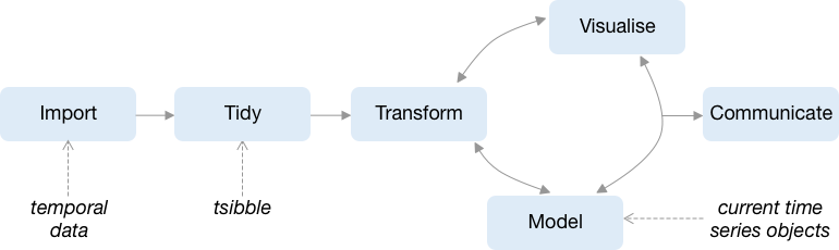
Figure 2: Where do temporal data, tsibble and current time series objects feed in the data science pipeline?
tsibble = key + index
We’re going to explore Citi bike trips in New York City, with the focus on temporal context. The dataset comprises 333,687 trips from January 2018 till November, each connecting to its bike id, duration, station’s geography and rider’s demography.
nycbikes18#> # A tibble: 333,687 x 15
#> tripduration starttime stoptime `start station …
#> <dbl> <dttm> <dttm> <dbl>
#> 1 932 2018-01-01 02:06:17 2018-01-01 02:21:50 3183
#> 2 550 2018-01-01 12:06:18 2018-01-01 12:15:28 3183
#> 3 510 2018-01-01 12:06:56 2018-01-01 12:15:27 3183
#> 4 354 2018-01-01 14:53:10 2018-01-01 14:59:05 3183
#> # … with 3.337e+05 more rows, and 11 more variables: `start station
#> # name` <chr>, `start station latitude` <dbl>, `start station
#> # longitude` <dbl>, `end station id` <dbl>, `end station name` <chr>,
#> # `end station latitude` <dbl>, `end station longitude` <dbl>,
#> # bikeid <dbl>, usertype <chr>, `birth year` <dbl>, gender <dbl>It arrives in the “melted” format, where each observation describes a trip event about a registered bike at a particular time point. Each bike (bikeid) is the observational unit that we’d like to study over time, forming the “key”; its starting time (starttime) provides the time basis. Whilst creating a tsibble, we have to declare the key and index. The data is all about events with irregularly spaced in time, thus specifying regular = FALSE.
library(tsibble)
library(tidyverse)
library(lubridate)
nycbikes_ts <- nycbikes18 %>%
  as_tsibble(key = bikeid, index = starttime, regular = FALSE)
A check with validate = TRUE is performed during the construction of a tsibble to validate if the key and index determine distinct rows. Duplicates signal a data quality issue, which would likely affect subsequent analyses and hence decision making. Users are encouraged to gaze at data early and reason the process of data cleaning. duplicates() helps to find identical key-index entries. Unique key-index pairs ensure a tsibble to be a valid input for time series analytics and models.
Some types of operation assume an input in a strict temporal order, such as lag(), lead() and difference(). Therefore the ordering of data rows is arranged in the first place by the key and then index from past to recent.
The print output of a tibble (yes, tibble, not tsibble) gives a quick glimpse at the data, and the tsibble’s print method adds more contextual information. Alongside the data dimension, we are informed by the time interval ([!] for irregularity) and index’s time zone if it’s POSIXct; the “key” variables are reported, with the number of units in the data. 900 bikes have served 333,687 trips in 2018. Displaying time zones is useful too, because time zones associated with POSIXct are concealed in data frames. Time zone is a critical piece when manipulating time. Especially, the data time zone is neither “UTC” nor my local time zone (“Australia/Melbourne”). When parsing characters to date-times, lubridate functions (such as ymd_hms()) default to “UTC” whereas base functions (such as as.POSIXct()) sets to local time zone.
nycbikes_ts#> # A tsibble: 333,687 x 15 [!] <America/New_York>
#> # Key: bikeid [900]
#> tripduration starttime stoptime `start station …
#> <dbl> <dttm> <dttm> <dbl>
#> 1 164 2018-11-21 07:16:03 2018-11-21 07:18:48 3279
#> 2 116 2018-11-21 09:59:10 2018-11-21 10:01:06 3272
#> 3 115 2018-11-22 06:51:08 2018-11-22 06:53:04 3273
#> 4 135 2018-11-23 09:59:57 2018-11-23 10:02:13 3272
#> # … with 3.337e+05 more rows, and 11 more variables: `start station
#> # name` <chr>, `start station latitude` <dbl>, `start station
#> # longitude` <dbl>, `end station id` <dbl>, `end station name` <chr>,
#> # `end station latitude` <dbl>, `end station longitude` <dbl>,
#> # bikeid <dbl>, usertype <chr>, `birth year` <dbl>, gender <dbl>Column-wise tidyverse verbs
Tsibble is essentially a tibble with extra contextual semantics: key and index. The tidyverse methods can be naturally applied to a tsibble. Row-wise verbs, for example filter() and arrange(), work for a tsibble in exactly the same way as a general data frame, but column-wise verbs behave differently yet intentionally.
- The index column cannot be dropped.
nycbikes_ts %>%
select(-starttime)#> Column `starttime` (index) can't be removed.
#> Do you need `as_tibble()` to work with data frame?- Column selection always includes the index. Explicitly selecting the index will suppress the message.
nycbikes_ts %>%
select(bikeid, tripduration)#> Selecting index: "starttime"#> # A tsibble: 333,687 x 3 [!] <America/New_York>
#> # Key: bikeid [900]
#> bikeid tripduration starttime
#> <dbl> <dbl> <dttm>
#> 1 14697 164 2018-11-21 07:16:03
#> 2 14697 116 2018-11-21 09:59:10
#> 3 14697 115 2018-11-22 06:51:08
#> 4 14697 135 2018-11-23 09:59:57
#> # … with 3.337e+05 more rows- Modifying the key variable may result in an invalid tsibble, thus issuing an error.
nycbikes_ts %>%
  mutate(bikeid = 2018L)
#> The result is not a valid tsibble.
#> Do you need `as_tibble()` to work with data frame?- Summarising a tsibble reduces to a sequence of unique time points instead of a single value.
nycbikes_ts %>%
summarise(ntrip = n())#> # A tsibble: 333,682 x 2 [!] <America/New_York>
#> starttime ntrip
#> <dttm> <int>
#> 1 2018-01-01 00:01:45 1
#> 2 2018-01-01 01:27:17 1
#> 3 2018-01-01 01:29:03 1
#> 4 2018-01-01 01:59:31 1
#> # … with 3.337e+05 more rowsIf a tsibble cannot be maintained in the output of a pipeline module, for example the index is dropped, an error informs users of the problem and suggests alternatives. This avoids negatively surprising users and reminds them of time context.
New time-based verbs
A few new verbs are introduced to make time-aware manipulation a little easier. One of the frequently used operations is subsetting time window. If multiple time windows (for example winter and summer months) are to be picked, we have to set time zones and figure out where to put | and & if using dplyr filter().
tzone <- "America/New_York"
nycbikes_ts %>%
  filter(
    starttime <= ymd("2018-02-28", tz = tzone) |
    starttime >= ymd("2018-07-01", tz = tzone),
    starttime <= ymd("2018-08-31", tz = tzone)
  )
Tsibble knows the index coupled with time zone, and thereby a shorthand filter_index() is for conveniently filtering time. Initially I was hesitant to add this feature, but it is too verbose when involving time zone specification. The resulting equivalent saves us a few keystrokes without losing much expressiveness.
nycbikes_ts %>%
filter_index(~ "2018-02", "2018-07" ~ "2018-08")#> # A tsibble: 114,481 x 15 [!] <America/New_York>
#> # Key: bikeid [787]
#> tripduration starttime stoptime `start station …
#> <dbl> <dttm> <dttm> <dbl>
#> 1 1646 2018-08-16 20:19:52 2018-08-16 20:47:19 3192
#> 2 503 2018-08-17 07:44:28 2018-08-17 07:52:52 3192
#> 3 212 2018-08-17 10:06:06 2018-08-17 10:09:39 3186
#> 4 485 2018-08-18 11:08:00 2018-08-18 11:16:06 3483
#> # … with 1.145e+05 more rows, and 11 more variables: `start station
#> # name` <chr>, `start station latitude` <dbl>, `start station
#> # longitude` <dbl>, `end station id` <dbl>, `end station name` <chr>,
#> # `end station latitude` <dbl>, `end station longitude` <dbl>,
#> # bikeid <dbl>, usertype <chr>, `birth year` <dbl>, gender <dbl>This event data needs some aggregation to be more informative. It is common to aggregate to less granular time intervals for temporal data. index_by() provides the means to prepare grouping for time index by calling an arbitrary function to the index. Lubridate’s functions such as floor_date(), celling_date() and round_date() are helpful to do all sorts of sub-daily rounding; as_date() and year() help transit to daily and annual numbers respectively. yearweek(), yearmonth() and yearquarter() in the tsibble cover other time ranges. Here we are interested in hourly tallies using floor_date(). As you may notice, the new variable starthour is part of groupings, prefixed by @.
nycbikes_ts %>%
index_by(starthour = floor_date(starttime, unit = "1 hour"))#> # A tsibble: 333,687 x 16 [!] <America/New_York>
#> # Key: bikeid [900]
#> # Groups: @ starthour [7,648]
#> tripduration starttime stoptime `start station …
#> <dbl> <dttm> <dttm> <dbl>
#> 1 164 2018-11-21 07:16:03 2018-11-21 07:18:48 3279
#> 2 116 2018-11-21 09:59:10 2018-11-21 10:01:06 3272
#> 3 115 2018-11-22 06:51:08 2018-11-22 06:53:04 3273
#> 4 135 2018-11-23 09:59:57 2018-11-23 10:02:13 3272
#> # … with 3.337e+05 more rows, and 12 more variables: `start station
#> # name` <chr>, `start station latitude` <dbl>, `start station
#> # longitude` <dbl>, `end station id` <dbl>, `end station name` <chr>,
#> # `end station latitude` <dbl>, `end station longitude` <dbl>,
#> # bikeid <dbl>, usertype <chr>, `birth year` <dbl>, gender <dbl>,
#> # starthour <dttm>In spirit of group_by(), index_by() takes effect in conjunction with succeeding operations for example summarise(). The following snippet is how we achieve in computing the number of trips every hour. Have you noticed that the displayed interval switches from irregular [!] to one hour [1h]?
hourly_trips <- nycbikes_ts %>%
  index_by(starthour = floor_date(starttime, unit = "1 hour")) %>%
  summarise(ntrips = n()) %>%
print()#> # A tsibble: 7,648 x 2 [1h] <America/New_York>
#> starthour ntrips
#> <dttm> <int>
#> 1 2018-01-01 00:00:00 1
#> 2 2018-01-01 01:00:00 3
#> 3 2018-01-01 02:00:00 3
#> 4 2018-01-01 03:00:00 7
#> # … with 7,644 more rowsThere are a handful of functions for handling implicit missing values, all suffixed with _gaps():
has_gaps()checks if there exists implicit missingness.scan_gaps()reports all implicit missing observations.count_gaps()summarises the time ranges that are absent from the data.fill_gaps()turns them into explicit ones, along with filling in gaps by values or functions.
The majority of time gaps congregate between 1am and 5am. We should be able to conclude that the data is not recorded because of no bike use.
scan_gaps(hourly_trips) %>%
  print() %>%
  mutate(time = hour(starthour)) %>%
  ggplot(aes(x = time)) +
geom_bar()#> # A tsibble: 368 x 1 [1h] <America/New_York>
#> starthour
#> <dttm>
#> 1 2018-01-01 05:00:00
#> 2 2018-01-01 07:00:00
#> 3 2018-01-01 23:00:00
#> 4 2018-01-02 01:00:00
#> # … with 364 more rows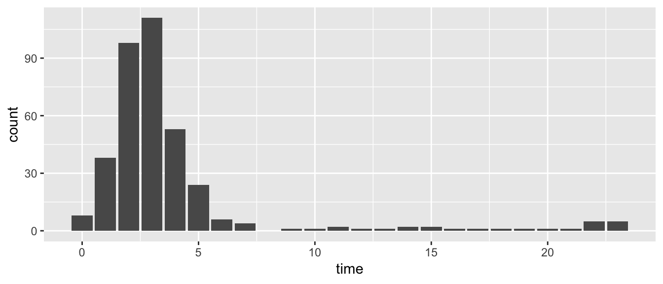
Filling in gaps with ntrips = 0L gives us a complete tsibble, otherwise NA for gaps in ntrips.
full_trips <- hourly_trips %>%
  fill_gaps(ntrips = 0L)
Hourly tallies for winter and summer months are laid out in the calendar format using sugrrants::facet_calendar(). The bike usage is primarily driven by commuters in working days. The pattern on July 4th pops out like a weekend due to Independence day in US. No surprise, New Yorkers bike more in summer than winter time.
full_trips %>%
  filter_index(~ "2018-02", "2018-07" ~ "2018-08") %>%
  mutate(date = as_date(starthour), time = hour(starthour)) %>%
  ggplot(aes(x = time, y = ntrips)) +
  geom_line() +
  sugrrants::facet_calendar(~ date) +
  scale_x_continuous(breaks = c(6, 18))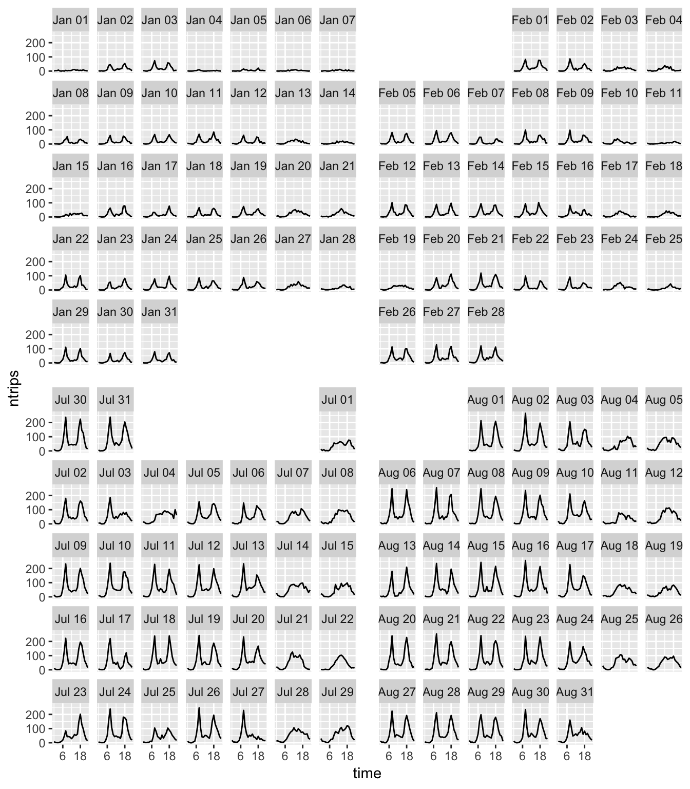
When a tsibble is set up, it takes care of updating key and index throughout the pipeline. Will two user groups, customers and subscribers, have different bike trip histories during a day? The interested subjects shift from every single bike bikeid to each user type usertype.
usertype_ts <- nycbikes_ts %>%
  group_by(usertype) %>%
  index_by(hour = hour(starttime)) %>%
  summarise(
    avg_tripd = mean(tripduration),
    ntrips = n()
  ) %>%
print()#> # A tsibble: 48 x 4 [1]
#> # Key: usertype [2]
#> usertype hour avg_tripd ntrips
#> <chr> <int> <dbl> <int>
#> 1 Customer 0 3223. 233
#> 2 Customer 1 3727. 143
#> 3 Customer 2 12099. 120
#> 4 Customer 3 15008. 53
#> # … with 44 more rowsCiti bike members commute more frequently with bikes for short distance, whereas one-time customers tend to travel for a longer period but ride much less.
library(patchwork)
p1 <- usertype_ts %>%
  ggplot(aes(x = hour, y = ntrips, colour = usertype)) +
  geom_point() +
  geom_line(aes(group = usertype)) +
  theme(legend.position = "none")
p2 <- usertype_ts %>%
  ggplot(aes(x = hour, y = avg_tripd, colour = usertype)) +
  geom_point() +
  geom_line(aes(group = usertype))
p1 + p2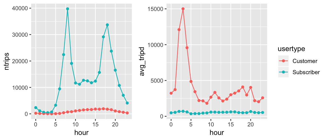
Ending
A large chunk of tsibble’s functions that are dedicated to performing rolling window operations are left untouched in this post. You may like to read more about rolling window here.
I have added parallel support to them in v0.6.2, prefixed with future_ (like future_slide()) by taking advantage of the awesome furrr package.
The tsibble package forms the infrastructure for new forecasting software, fable. I will be speaking about a streamlined workflow for tidy time series analysis, including forecasting tsibble (goodbye to ts) at rstudio::conf in January.
(last updated: “2019-05-04”)