Calibrating time zones: an early bird or a night owl?

I studied my step data while in self-quarantine, and happened to fell into the time zone trap. The #twofunctions in lubridate are the rescuers: with_tz() and force_tz().

library(tidyverse)
library(lubridate)

The first lines of data say: I’m not a night 🦉, but 👻 wandering through the dark.

#> # A tibble: 5,458 x 2
#>    date_time           count
#>    <dttm>              <dbl>
#>  1 2018-12-31 03:00:00    26
#>  2 2018-12-31 11:00:00    11
#>  3 2018-12-31 22:00:00   764
#>  4 2018-12-31 23:00:00   913
#>  5 2019-01-01 13:00:00     9
#>  6 2019-01-01 23:00:00  2910
#>  7 2019-01-02 00:00:00  1390
#>  8 2019-01-02 01:00:00  1020
#>  9 2019-01-02 02:00:00   472
#> 10 2019-01-02 04:00:00  1220
#> # … with 5,448 more rows

---

The story begins with data exported in UTC and read to UTC by default. But the compact data display doesn’t speak of time zone, and we have to get it unpacked to find out.

tz(step_count[["date_time"]])

#> [1] "UTC"

The with_tz() turns the clock to a new time zone, and shifts my life back to normal.

step_count <- step_count %>% 
  mutate(date_time = with_tz(date_time, tzone = "Australia/Melbourne")) %>% 
  filter(year(date_time) == 2019)
step_count

#> # A tibble: 5,448 x 2
#>    date_time           count
#>    <dttm>              <dbl>
#>  1 2019-01-01 09:00:00   764
#>  2 2019-01-01 10:00:00   913
#>  3 2019-01-02 00:00:00     9
#>  4 2019-01-02 10:00:00  2910
#>  5 2019-01-02 11:00:00  1390
#>  6 2019-01-02 12:00:00  1020
#>  7 2019-01-02 13:00:00   472
#>  8 2019-01-02 15:00:00  1220
#>  9 2019-01-02 16:00:00  1670
#> 10 2019-01-02 17:00:00  1390
#> # … with 5,438 more rows

My eyebrows rise in surprise again: I’m probably 👻 from time to time.

step_count %>% 
  ggplot(aes(x = hour(date_time), y = count)) +
  geom_jitter(position = position_jitter(0.3, seed = 2020), alpha = 0.5) +
  stat_summary(fun.data = mean_cl_boot, geom = "pointrange", color = "red") +
  xlab("time")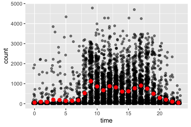

The calendar plot (beyond heatmap) is an exploratory visualisation tool for quickly eyeballing the overalls and locating the spooky ones. The ghostly movements I found actually correspond to my conference trips last year: rstudio::conf(2019L) and JSM.

austin <- seq(ymd("2019-01-15"), ymd("2019-01-25"), by = "1 day")
denver <- seq(ymd("2019-07-28"), ymd("2019-08-01"), by = "1 day")
sf <- seq(ymd("2019-08-02"), ymd("2019-08-06"), by = "1 day")

library(sugrrants)
step_cal <- step_count %>% 
  complete(date_time = full_seq(date_time, 3600), fill = list(count = 0)) %>% 
  mutate(
    hour = hour(date_time), 
    date = as_date(date_time),
    overseas = ifelse(date %in% c(austin, denver, sf), "overseas", "local")
  ) %>% 
  frame_calendar(x = hour, y = count, date = date)
p_cal <- step_cal %>% 
  ggplot(aes(x = .hour, y = .count, group = date, colour = overseas)) +
  geom_line()
prettify(p_cal) + theme(legend.position = "bottom")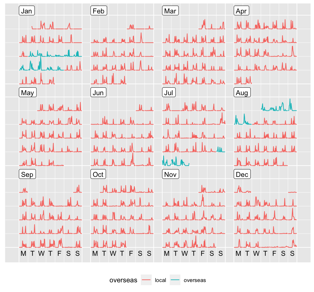

Time zones can be silent contaminators, if we don’t look at the data. Jet lag can’t disrupt my sleep that badly. The clock in those travel days should be turned around with with_tz(), but R inhibits multiple time zones passed to a single date-time vector. Here the force_tz() comes to rescue: keep the clock as is but overwritten with new time zone. The floating times are pushed back to where they should be (with_tz()), and get frozen in a unified time zone (force_tz()).

lock_local_time <- function(x, tz) {
  force_tz(with_tz(x, tz = tz), tzone = "Australia/Melbourne")
}

local_step_count <- step_count %>% 
  mutate(
    date = as_date(date_time),
    date_time = case_when(
      date %in% austin ~ lock_local_time(date_time, tz = "US/Central"),
      date %in% denver ~ lock_local_time(date_time, tz = "US/Mountain"),
      date %in% sf ~ lock_local_time(date_time, tz = "US/Pacific"),
      TRUE ~ date_time
    )
  )

local_step_count %>% 
  ggplot(aes(x = hour(date_time), y = count)) +
  geom_jitter(position = position_jitter(0.3, seed = 2020), alpha = 0.5) +
  stat_summary(fun.data = mean_cl_boot, geom = "pointrange", color = "red") +
  xlab("time")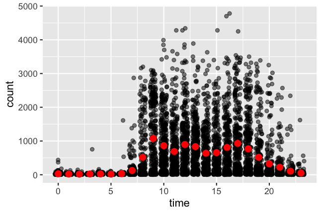

Phew, the data finally makes sense: neither an early bird, nor a night owl. But the message is clear that I was determined to get my PhD done, because I held on to a routine (on average)! 😂